#Multiplication of Vector By Scalars

[sunless-not-sinless]

oh boy those are not the last. it goes up. a lot. and each time you lose something

adding i means you lose the property that x^2≥0 ofc. you also lose order. z<w makes no sense in two dimensions

adding j and k means you lose commutivity. a*b is not necessarily b*a.

going from four to eight dimensions you lose associativity. a*(b*c) is not necessarily (a*b)*c. at this point you also stop calling them i, j, and k because you would be using too many letters.

but there is some structure. x*(x*y)=(x*x)*y, and (y*x)*x=y*(x*x)

moving to 16 dimensions now and you lose this property

you also lose division.

at 16 dimensions we have now lost an entire operation instead of properties of these operations

[prokopetz]

While we're talking about AnyDice, do you know if there's a way to accurately test the probability of multiple outcomes on unconventional dice? The below link is an abriged test of an implementation of FFG's Genesys dice I found on a forum thread; the tester was trying to work out if the implementation was even correct, and testing for 2 Advantages AND two Successes on one ability dice (which is impossible, but AnyDice gives 1.56%). The ability dice is a d8; only one side has 2A and only one side has 2S, and they're different sides. The intuition is that because the advantage sides and the successes sides are defined in different orders, the same index for success and advantage should be used which will never see a 2 on both arrays. AnyDice just outputs the intersection of the two 1-in-8s, 1/64 = 0.015625. Do you know of any way to get the intuitive output, or is this just a reflection of AnyDice being a probability calculator and not a dice roller? https://anydice.com/program/3aeb3

Yeah, no, that's completely wrong. What you've got there is is a script to generate the results of rolling two dice, one of which has only success symbols and no advantage symbols, and the other of which has only advantage symbols and no success symbols. That's where your unexpected intersection is coming from.

The problem here is that, because each die can have multiple kinds of symbols on it, potentially including multiple kinds of symbols on a single face, and we care about the total number of each kind of symbol, our odds become a sum of vectors rather than a sum of scalars. I'm not aware of any widely available dice probability calculator that can elegantly handle dice which produce vector results.

We can cheat a bit in this particular case, though, because the fact that we don't need to deal with negative numbers means we can convert a vector result to a scalar result by assigning each symbol a power of ten.

For the sake of argument, let's assign each "success" a value of 10, and each "advantage" a value of one. Thus, a face with one "success" symbol becomes a 10; a face with two "success" symbols, a 20; a face with one "success" and one "advantage", an 11; and so forth.

In the table of results, we then examine the digits individually, with the "tens" place being read as the number of success symbols, and the "ones" place being read as the number of advantage symbols.

Expressed in this way in AnyDice terms, a Genesys skill die becomes:

output 1d{0, 10, 10, 20, 1, 1, 11, 2}

In the resulting table, you'll see that your anomalous intersection has vanished; there's a 12.5% chance of "2" (that is, two advantages with zero successes), and a 12.5% chance of "20" (two successes with zero advantages), but no "22" (two successes with two advantages).

Note, however, that this only works correctly with up to four dice; with five or more, there will be some outcomes where the number of advantage symbols exceeds nine and "overflows" into the successes column, polluting your results.

Clear as mud?

[jbfly46]

̲𝚄̲̲𝚗̲̲𝚒̲̲𝚟̲̲𝚎̲̲𝚛̲̲𝚜̲̲𝚊̲̲𝚕̲ ̲𝙸̲̲𝚗̲̲𝚎̲̲𝚚̲̲𝚞̲̲𝚊̲̲𝚕̲̲𝚒̲̲𝚝̲̲𝚒̲̲𝚎̲̲𝚜̲

Jensen’s Inequality:

If φ is a convex function and X is a random variable, then:

φ(E[X]) ≤ E[φ(X])

⸻

- Mathematically:

It formalizes the idea that the function of an average is less than or equal to the average of the function—a cornerstone in information theory, economics, and entropy models.

- Philosophically:

It encodes a deep truth about aggregation vs individuality:

The average path does not capture the richness of individual variation.

You can’t just compress people, ideas, or experiences into a mean and expect to preserve their depth.

- Theologically (Logos lens):

God doesn’t save averages. He saves individuals.

Jensen’s Inequality reminds us: truth emerges not from flattening, but from preserving the shape of each curve.

Cauchy-Schwarz Inequality:

|⟨u, v⟩| ≤ ||u|| · ||v||

- Meaning:

The inner product (projection) of two vectors is always less than or equal to the product of their lengths.

- Why it matters metaphysically:

No interaction (⟨u,v⟩) can exceed the potential of its participants (||u||, ||v||).

Perfect alignment (equality) happens only when one vector is a scalar multiple of the other—i.e., they share direction.

- Philosophical resonance:

Love (inner product) can never exceed the strength of self and other—unless they are one in direction.

⸻

Triangle Inequality

||x + y|| ≤ ||x|| + ||y||

- Meaning:

The shortest path between two points is not through combining detours.

- Metaphysical translation:

Every time you try to shortcut wholeness by adding parts, you risk increasing the distance.

Truth is straight. But sin adds loops.

This is why grace cuts cleanly—it does not add noise.

⸻

Entropic Inequality (Data Processing Inequality):

I(X; Y) ≥ I(f(X); Y)

- Meaning:

You can’t increase information about a variable by processing it. Filtering always loses some signal.

- Deep translation:

Every time you mediate the truth through an agenda, a platform, or an ego, you lose information.

This is a law of entropy and a law of theology.

“Now we see through a glass, darkly…”

—1 Corinthians 13:12

Only unfiltered presence (Logos) sees all.

⸻

Christic Inequality (Cruciform Principle):

Here’s a theological-metaphysical inequality you won’t find in a textbook:

Power - Sacrifice ≤ 0

(unless crucified)

- Meaning:

Power without self-giving always decays into corruption.

Only when power is poured out (Philippians 2:6–8) does it become greater than itself.

So paradoxically:

True Power = Power · (Sacrifice > 0)

[bubbloquacious]

8. Least favorite notation you’ve ever seen?

12. Who actually invented calculus?

52. Do you have favorite math textbooks? If so, what are they?

57. What inspired you to do math?

:)))

From Real's Math Ask Meme.

8. Least favourite notation you’ve ever seen?

Writing a tensor product of bra-ket vectors as |1⟩|2⟩ instead of |1⟩⊗|2⟩, which was standard in the quantum information theory course I took (with @floralfractals :^)) a few years back. This makes an expression like ⟨1|⟨2||3⟩|4⟩ ambiguous! It evaluates to ⟨1|3⟩⟨2|4⟩ if you interpret the juxtaposition as a tensor product, and to ⟨1|4⟩⟨2|3⟩ if you intepret it as scalar multiplication.

10. Who actually invented calculus?

I did! Or I will have done, when I invent my time machine to travel back to the Islamic Golden Age to tell Al-Khwarizmi about category theory. Then they'll all see.

44. Do you have favourite math textbooks? If so, what are they?

I never stick with textbooks long enough for these to be like super well-founded recommendations, but I quite like Jonathan Gleason's Introduction to Analysis, Peter Johnstone's Stone Spaces, and Bochnak, Coste, & Roy's Real Algebraic Geometry.

49. What inspired you to do math?

So besides the fact that from a young age I was intrigued and engaged by puzzles and problem solving, it took quite some time before I realized I wanted to become a mathematician. Sometime during my fourth or fifth year of secondary school we covered logarithms, and that's when it all started to click for me. How addition, multiplication, exponentiation are just operations, and that they can have inverse operations, and that these are all examples of the exact same phenomenon. I started watching Vsauce and Numberphile and Vihart, and the rest is history.

[eka-mark]

Here's a helpful and elementary perspective on ideals of rings that I recently picked up from some of Richard Borcherds's lectures on YouTube: an ideal of R is a submodule of R (thought of as a free module over itself).

The defining properties of an ideal are being an abelian subgroup of (R,+) and being closed under ("scalar") multiplication by elements of R. Those are just the defining properties of a subspace of a vector space!

Think about a field as a 1-dimensional vector space over itself. It has no nontrivial proper subspaces, and this is exactly the same as the fact that a field has no nontrivial proper ideals (just the 0 ideal and the whole field). Finitely-generated modules over a general ring don't have this nice stratification by dimension, so a free R-module on one generator may have nontrivial proper submodules ("nontrivial proper subspaces of a 1-dimensional module").

For example, there's no subset of the real line that's closed under addition and (real) scalar multiplication, but Z has the perfectly nice subset 2Z with the corresponding properties.

[enetarch-quantum-physics]

Topics to study for Quantum Physics

Calculus

Taylor Series

Sequences of Functions

Transcendental Equations

Differential Equations

Linear Algebra

Separation of Variables

Scalars

Vectors

Matrixes

Operators

Basis

Vector Operators

Inner Products

Identity Matrix

Unitary Matrix

Unitary Operators

Evolution Operator

Transformation

Rotational Matrix

Eigen Values

Coefficients

Linear Combinations

Matrix Elements

Delta Sequences

Vectors

Basics

Derivatives

Cartesian

Polar Coordinates

Cylindrical

Spherical

LaPlacian

Generalized Coordinate Systems

Waves

Components of Equations

Versions of the equation

Amplitudes

Time Dependent

Time Independent

Position Dependent

Complex Waves

Standing Waves

Nodes

AntiNodes

Traveling Waves

Plane Waves

Incident

Transmission

Reflection

Boundary Conditions

Probability

Probability

Probability Densities

Statistical Interpretation

Discrete Variables

Continuous Variables

Normalization

Probability Distribution

Conservation of Probability

Continuum Limit

Classical Mechanics

Position

Momentum

Center of Mass

Reduce Mass

Action Principle

Elastic and Inelastic Collisions

Physical State

Waves vs Particles

Probability Waves

Quantum Physics

Schroedinger Equation

Uncertainty Principle

Complex Conjugates

Continuity Equation

Quantization Rules

Heisenburg's Uncertianty Principle

Schroedinger Equation

TISE

Seperation from Time

Stationary States

Infinite Square Well

Harmonic Oscillator

Free Particle

Kronecker Delta Functions

Delta Function Potentials

Bound States

Finite Square Well

Scattering States

Incident Particles

Reflected Particles

Transmitted Particles

Motion

Quantum States

Group Velocity

Phase Velocity

Probabilities from Inner Products

Born Interpretation

Hilbert Space

Observables

Operators

Hermitian Operators

Determinate States

Degenerate States

Non-Degenerate States

n-Fold Degenerate States

Symetric States

State Function

State of the System

Eigen States

Eigen States of Position

Eigen States of Momentum

Eigen States of Zero Uncertainty

Eigen Energies

Eigen Energy Values

Eigen Energy States

Eigen Functions

Required properties

Eigen Energy States

Quantification

Negative Energy

Eigen Value Equations

Energy Gaps

Band Gaps

Atomic Spectra

Discrete Spectra

Continuous Spectra

Generalized Statistical Interpretation

Atomic Energy States

Sommerfels Model

The correspondence Principle

Wave Packet

Minimum Uncertainty

Energy Time Uncertainty

Bases of Hilbert Space

Fermi Dirac Notation

Changing Bases

Coordinate Systems

Cartesian

Cylindrical

Spherical - radii, azmithal, angle

Angular Equation

Radial Equation

Hydrogen Atom

Radial Wave Equation

Spectrum of Hydrogen

Angular Momentum

Total Angular Momentum

Orbital Angular Momentum

Angular Momentum Cones

Spin

Spin 1/2

Spin Orbital Interaction Energy

Electron in a Magnetic Field

ElectroMagnetic Interactions

Minimal Coupling

Orbital magnetic dipole moments

Two particle systems

Bosons

Fermions

Exchange Forces

Symmetry

Atoms

Helium

Periodic Table

Solids

Free Electron Gas

Band Structure

Transformations

Transformation in Space

Translation Operator

Translational Symmetry

Conservation Laws

Conservation of Probability

Parity

Parity In 1D

Parity In 2D

Parity In 3D

Even Parity

Odd Parity

Parity selection rules

Rotational Symmetry

Rotations about the z-axis

Rotations in 3D

Degeneracy

Selection rules for Scalars

Translations in time

Time Dependent Equations

Time Translation Invariance

Reflection Symmetry

Periodicity

Stern Gerlach experiment

Dynamic Variables

Kets, Bras and Operators

Multiplication

Measurements

Simultaneous measurements

Compatible Observable

Incompatible Observable

Transformation Matrix

Unitary Equivalent Observable

Position and Momentum Measurements

Wave Functions in Position and Momentum Space

Position space wave functions

momentum operator in position basis

Momentum Space wave functions

Wave Packets

Localized Wave Packets

Gaussian Wave Packets

Motion of Wave Packets

Potentials

Zero Potential

Potential Wells

Potentials in 1D

Potentials in 2D

Potentials in 3D

Linear Potential

Rectangular Potentials

Step Potentials

Central Potential

Bound States

UnBound States

Scattering States

Tunneling

Double Well

Square Barrier

Infinite Square Well Potential

Simple Harmonic Oscillator Potential

Binding Potentials

Non Binding Potentials

Forbidden domains

Forbidden regions

Quantum corral

Classically Allowed Regions

Classically Forbidden Regions

Regions

Landau Levels

Quantum Hall Effect

Molecular Binding

Quantum Numbers

Magnetic

Withal

Principle

Transformations

Gauge Transformations

Commutators

Commuting Operators

Non-Commuting Operators

Commutator Relations of Angular Momentum

Pauli Exclusion Principle

Orbitals

Multiplets

Excited States

Ground State

Spherical Bessel equations

Spherical Bessel Functions

Orthonormal

Orthogonal

Orthogonality

Polarized and UnPolarized Beams

Ladder Operators

Raising and Lowering Operators

Spherical harmonics

Isotropic Harmonic Oscillator

Coulomb Potential

Identical particles

Distinguishable particles

Expectation Values

Ehrenfests Theorem

Simple Harmonic Oscillator

Euler Lagrange Equations

Principle of Least Time

Principle of Least Action

Hamilton's Equation

Hamiltonian Equation

Classical Mechanics

Transition States

Selection Rules

Coherent State

Hydrogen Atom

Electron orbital velocity

principal quantum number

Spectroscopic Notation

=====

Common Equations

Energy (E) .. KE + V

Kinetic Energy (KE) .. KE = 1/2 m v^2

Potential Energy (V)

Momentum (p) is mass times velocity

Force equals mass times acceleration (f = m a)

Newtons' Law of Motion

Wave Length (λ) .. λ = h / p

Wave number (k) ..

k = 2 PI / λ

= p / h-bar

Frequency (f) .. f = 1 / period

Period (T) .. T = 1 / frequency

Density (λ) .. mass / volume

Reduced Mass (m) .. m = (m1 m2) / (m1 + m2)

Angular momentum (L)

Waves (w) ..

w = A sin (kx - wt + o)

w = A exp (i (kx - wt) ) + B exp (-i (kx - wt) )

Angular Frequency (w) ..

w = 2 PI f

= E / h-bar

Schroedinger's Equation

-p^2 [d/dx]^2 w (x, t) + V (x) w (x, t) = i h-bar [d/dt] w(x, t)

-p^2 [d/dx]^2 w (x) T (t) + V (x) w (x) T (t) = i h-bar [d/dt] w(x) T (t)

Time Dependent Schroedinger Equation

[ -p^2 [d/dx]^2 w (x) + V (x) w (x) ] / w (x) = i h-bar [d/dt] T (t) / T (t)

E w (x) = -p^2 [d/dx]^2 w (x) + V (x) w (x)

E i h-bar T (t) = [d/dt] T (t)

TISE - Time Independent

H w = E w

H w = -p^2 [d/dx]^2 w (x) + V (x) w (x)

H = -p^2 [d/dx]^2 + V (x)

-p^2 [d/dx]^2 w (x) + V (x) w (x) = E w (x)

Conversions

Energy / wave length ..

E = h f

E [n] = n h f

= (h-bar k[n])^2 / 2m

= (h-bar n PI)^2 / 2m

= sqr (p^2 c^2 + m^2 c^4)

Kinetic Energy (KE)

KE = 1/2 m v^2

= p^2 / 2m

Momentum (p)

p = h / λ

= sqr (2 m K)

= E / c

= h f / c

Angular momentum ..

p = n h / r, n = [1 .. oo] integers

Wave Length ..

λ = h / p

= h r / n (h / 2 PI)

= 2 PI r / n

= h / sqr (2 m K)

Constants

Planks constant (h)

Rydberg's constant (R)

Avogadro's number (Na)

Planks reduced constant (h-bar) .. h-bar = h / 2 PI

Speed of light (c)

electron mass (me)

proton mass (mp)

Boltzmann's constant (K)

Coulomb's constant

Bohr radius

Electron Volts to Jules

Meter Scale

Gravitational Constant is 6.7e-11 m^3 / kg s^2

History of Experiments

Light

Interference

Diffraction

Diffraction Gratings

Black body radiation

Planks formula

Compton Effect

Photo Electric Effect

Heisenberg's Microscope

Rutherford Planetary Model

Bohr Atom

de Broglie Waves

Double slit experiment

Light

Electrons

Casmir Effect

Pair Production

Superposition

Schroedinger's Cat

EPR Paradox

Examples

Tossing a ball into the air

Stability of the Atom

2 Beads on a wire

Plane Pendulum

Wave Like Behavior of Electrons

Constrained movement between two concentric impermeable spheres

Rigid Rod

Rigid Rotator

Spring Oscillator

Balls rolling down Hill

Balls Tossed in Air

Multiple Pullys and Weights

Particle in a Box

Particle in a Circle

Experiments

Particle in a Tube

Particle in a 2D Box

Particle in a 3D Box

Simple Harmonic Oscillator

Scattering Experiments

Diffraction Experiments

Stern Gerlach Experiment

Rayleigh Scattering

Ramsauer Effect

Davisson–Germer experiment

Theorems

Cauchy Schwarz inequality

Fourier Transformation

Inverse Fourier Transformation

Integration by Parts

Terminology

Levi Civita symbol

Laplace Runge Lenz vector

[building-made-of-paper]

It's worse than that. Cows don't have to add together in the way we expect. As long as you can add cows together and multiply them by scalars and the output is always a cow, you have a vector space. But you can fuck with the definition of addition and multiplication (to a point) to make that work.

He's right tho

[mesmericmonad]

Chapter 10 in Part 2 of Process and Reality by Alfred North Whitehead. Probably the singular most exciting and sophisticated passages I've ever read

Whitehead here introduces two poles of identity philosophy that runs through the Western tradition: movement or stasis. dynamic becoming or static being.

Whitehead further examines the notion of "flux" and the relationship of movement in the universe to consciousness with brief remarks on Plato, Hume, Aristotle, Descartes, and Bergson

Whitehead suggests that Western philosophy discovered but never made conscious of the discovery that there are actually two kinds of fluency in the world: the microcosm and the macrocosm. The flowing inward of the Many into the unique, novel One, and the flowing outward of the One into the Many. Concrescence is the name for this process of subjective novelty and unification within the diverse Universe

"Concrescence is the name for the process in which the universe of many things acquires an individual unity in a determinate relegation of each item of the Many to its subordination in the constitution of the novel One." So far as an actual occasion is analyzable into component parts, this includes a process of feeling constituting (1) the actual occasions felt; (2) the eternal objects felt; (3) the feelings felt; (4) Its own subjective forms of intensity culminating in a satisfaction: "This final unity is termed the tsatisfaction.' The satisfaction is the culmination of the concrescence into a completely determinate matter of fact. In any of its antecedent stages, the concrescence exhibits sheer indetermination as to the nexus between its many components.

This multistage process is broken down even more by Whitehead into (i) the responsive phase and (ii) the supplemental stage, that leads us finally to the satisfaction. In the responsive phase, "the phase of pure reception of the actual world in its guise of objective datum for aesthetic synthesis. In this phase there is the mere reception of the actual world as a multiplicity of private centres of feeling, implicated in a nexus of mutual presupposition."

Whereas in the supplemental phase, "the many feelings, derivatively felt as alien, are transformed into a unity of aesthetic appreciation immediately felt as private. This is the incoming of appetition, which in its higher exemplifications we term vision. In the language of physical science, the scalar form overwhelms the original vector form: the origins become subordinate to the individual experience. The vector form is not lost, but is submerged as the foundation of the scalar superstructure."

In this next part, Whitehead breaks down the supplemental phase into two subphases: (1) aesthetic supplement; and (2) intellectual supplement. As he notes, if both subphases are trivial, the whole transmission of feelings passes through with little modification and augmentation. This part of the Concrescence urges in the dimensional axis of width of contrast and depth of intensity. "There is an emotional appreciation of the contrasts and rhythms inherent in the unification of the objective content in the concrescence" meaning that there is an actual felt sensation of differentiation of sense data with a gradation of consciousness of its vector origin. This elicits the second subphase: An eternal object realized in respect to its pure potentiality as related to determinate logical subjects is termed a 'propositional feeling' in the mentality of the actual occasion in question. The consciousness belonging to an actual occasion is its sub-phase of intellectual supplementation, when that sub-phase is not purely trivial. This sub-phase is the eliciting, into feeling, of the full contrast between mere propositional potentiality and realized fact."

Thus each actual entity, although complete so far as concerns its microscopic process, is yet incomplete by reason of its objective inclusion of the macroscopicprocess. It really experiences a future which must be actual, although the completed actualities of that future are undetermined. In this sense, each actual occasion experiences its own objective immortality.

[rickyabache]

Exporting data from R to different formats

Exporting data from R is a crucial step in sharing your analysis, reporting results, or saving processed data for future use. R provides a variety of functions and packages to export data into different formats, including CSV, Excel, JSON, and databases. This section will guide you through the process of exporting data from R into these various formats.

Exporting Data to CSV Files

CSV (Comma-Separated Values) files are one of the most common formats for sharing and storing tabular data. R makes it easy to export data frames to CSV using the write.csv() function.

Using write.csv():# Exporting a data frame to a CSV file write.csv(data, "path/to/save/your/file.csv", row.names = FALSE)

row.names = FALSE: This argument prevents row names from being written to the file, which is typically preferred when exporting data.

Customizing the Export:

You can further customize the CSV export by adjusting the delimiter, file encoding, and other options.# Exporting a data frame with custom settings write.csv(data, "path/to/save/your/file.csv", row.names = FALSE, sep = ";", fileEncoding = "UTF-8")

sep = ";": Changes the delimiter to a semicolon, which is common in some regions.

fileEncoding = "UTF-8": Ensures that the file is saved with UTF-8 encoding.

Exporting Data to Excel Files

Excel is widely used in business and academic environments. R provides several packages to export data to Excel, with openxlsx and writexl being popular options.

Using openxlsx:# Install and load the openxlsx package install.packages("openxlsx") library(openxlsx) # Exporting a data frame to an Excel file write.xlsx(data, "path/to/save/your/file.xlsx")

Using writexl:

The writexl package is another simple and efficient option for exporting data to Excel.# Install and load the writexl package install.packages("writexl") library(writexl) # Exporting a data frame to an Excel file write_xlsx(data, "path/to/save/your/file.xlsx")

Both of these methods allow for multiple sheets, formatting, and other advanced Excel features.

Exporting Data to JSON Files

JSON (JavaScript Object Notation) is a lightweight data-interchange format that is easy for both humans and machines to read and write. The jsonlite package in R makes exporting data to JSON straightforward.

Using jsonlite:# Install and load the jsonlite package install.packages("jsonlite") library(jsonlite) # Exporting a data frame to a JSON file write_json(data, "path/to/save/your/file.json")

Customizing the JSON Export:

You can customize the JSON structure by adjusting the pretty or auto_unbox arguments.# Exporting a data frame with custom settings write_json(data, "path/to/save/your/file.json", pretty = TRUE, auto_unbox = TRUE)

pretty = TRUE: Formats the JSON file with indentation for readability.

auto_unbox = TRUE: Converts single-element vectors to scalar JSON values.

Exporting Data to Databases

R can export data directly into databases, allowing for integration with larger data systems. The DBI package provides a standard interface for interacting with databases, and it works with specific database backend packages like RMySQL, RPostgreSQL, and RSQLite.

Using DBI with SQLite:# Install and load the DBI and RSQLite packages install.packages("DBI") install.packages("RSQLite") library(DBI) library(RSQLite) # Connecting to a SQLite database con <- dbConnect(RSQLite::SQLite(), dbname = "path/to/your/database.sqlite") # Exporting a data frame to a new table in the database dbWriteTable(con, "new_table_name", data) # Disconnecting from the database dbDisconnect(con)

This method can be adapted for other database systems by replacing RSQLite with the appropriate backend package (RMySQL, RPostgreSQL, etc.).

Exporting Data to Other Formats

In addition to CSV, Excel, JSON, and databases, R supports exporting data to various other formats such as:

Text Files: Using write.table() for general text-based formats.

SPSS, SAS, Stata: Using the haven package to export data to these formats.

HTML: Using the htmlTable package for exporting tables as HTML.

Example of Exporting to Text Files:# Exporting a data frame to a text file write.table(data, "path/to/save/your/file.txt", row.names = FALSE, sep = "\t")

sep = "\t": Specifies that the data should be tab-separated.

Best Practices for Data Export

File Naming: Use descriptive file names and include metadata such as dates or version numbers to keep track of different exports.

Check Data Integrity: Always verify that the exported data matches the original data, especially when working with non-CSV formats like JSON or Excel.

Automate Exports: For repeated tasks, consider writing functions or scripts to automate the export process, ensuring consistency and saving time.

Keep reading at strategic Leap

[complexbezier]

I don't have a complete answer to this anymore than anyone else, but the most satisfying hint towards an answer to the question "why do we have 3 spatial dimensions instead of some other number" that I have come accross is as follows:

If you take the postulates for quantum information theory (none of which say anything about spatial dimensions), and apply them to the simplest possible quantum system (a two-state quantum system or "qubit"), then you need 2 complex numbers to characterize the probability amplitudes of the two eigenstates of the system. Let's call these complex numbers A and B, amplitudes for the |on> and |off> states of the qubit respectively, so that we can write a state vector as A|on> + B|off>. Since each has a real and imaginary component (A=c+d*i, B=g+h*i), you can think of the overall quantum state of the system as having 4 degrees of freedom (c,d,g,h). So it lives in a "4d" space of possible states.

However, posssible states that differ only by an overall scalar multiple are considered physically indistinct: it is only the ratio between A and B that actually affects anything we can physically observe. So if you reduce this 4D space accordingly (first by eliminating distinctions in vector magnitude and then by eliminating distinctions of phase), you get a 3-sphere-surface of possible quantum states. This also means that there is also exactly a 3-sphere-surface of possible "observations" you could make on the system. Possible "ways" to observe the system, that is: because every mixed state of |on> and |off> is a valid eigenstate in some other observation basis (see "up" and "down" for spin). A spherical shell of possible observation operators thus exists, with the 3 Pauli x,y,z matrices serving as its generators. This sphere is sometimes called the "Bloch Sphere", and there's a good wikipedia page on it that you should check out if my explaination here sucks.

So, starting with only the formalism of quantum information theory, we've found that even for the simplest imaginable system, there needs to be a 3-sphere of distinct ways to observe it. One way this manifests physically is the electron spin--we need to first pick a direction in 3D space from which to observe it, before we can check whether it's "up" or "down" (a binary system that gains some spatial dimensionality due to its quantum nature).

To me personally, this is a convincing reason that something like a triad of spatial dimensions must exist in order for physical information to be observable. You could argue that maybe the 3 dimensions came first, and that the utility of complex numbers in quantum theory is a result of that, but I don't find this immensely convincing. After all, complex numbers represent the largest set of commutative numbers we could possibly use! (As far as I know anyway).

have they come up with a good reason for why reality has 3 dimensions

[teguhteja]

Vector Operations Python: Basic Mathematical inConcepts

Explore vector operations in Python with this comprehensive guide. Learn vector addition, scalar multiplication, and practical implementations using NumPy. Ideal for developers and data scientists

vector operations python, including vector addition and scalar multiplication, form the foundation of modern mathematical computing and data science. These fundamental concepts enable developers and data scientists to manipulate numerical data efficiently. Moreover, understanding these basic vector operations helps create powerful algorithms for machine learning applications. Understanding…

[marigold-22]

Tell me what a module is pelase

A module is a vector space over a ring instead of a field, if you don’t know what those words mean there are some great YouTube videos explaining it. A vector space is a space where things can be added and scaled by a field of scalars, a ring is a set with a notion of addition and multiplication, a field is a ring where multiplication is invertible. That’s probably the best I can do in one tumblr post, if you have any more specific questions I’ll try to explain them.

[bubbloquacious]

I read about an interesting incarnation of the hairy ball theorem recently. If you have a (unital) ring R and a (left) R-module M, then M is said to be stably free (of rank n - 1) if the direct sum M ⊕ R is isomorphic as an R-module to Rⁿ. This is more general than the property of being free (of rank n), which means that the module itself is isomorphic to Rⁿ, or equivalently that there is an n-element subset B (called a basis) of M such that every vector v ∈ M is a unique R-linear combination of elements of B.

Can we find stably free modules which are not free? For some common rings we cannot: stably free modules over any field, the integers, or any matrix ring over a field are always free. They do exist, though.

(First I should note that one thing that can go terribly wrong here is that there are rings out there such that the rank of a free module is not well-defined; there might be bases for the same module with a different number of elements. A ring where this doesn't happen has what's called the Invariant Basis Property (IBP). Luckily for us, all commutative rings have the IBP.)

Let S² denote the unit sphere in 3-dimensional Euclidean space, and let R be the ring of continuous functions S² -> ℝ. Consider the free R-module R³ whose elements are continuous vector-valued functions on S² . Let σ: R³ -> R be given by (f,g,h) ↦ x ⋅ f + y ⋅ g + z ⋅ h. This is a surjective module homomorphism because it maps (x,y,z) onto x² + y² + z² = 1 ∈ R. Then R³ is the internal direct sum of the kernel ker(σ) and the R-scalar multiples of (x,y,z). To see this, let (f,g,h) ∈ R³ be arbitrary. Then (f,g,h) = ((f,g,h) - σ(f,g,h) ⋅ (x,y,z)) + σ(f,g,h) ⋅ (x,y,z), so any element of R³ can be written as the sum of an element of ker(σ) and a multiple of (x,y,z) (this trick is essentially an application of the splitting lemma). It's also not terribly hard to prove that the intersection of ker(σ) and R ⋅ (x,y,z) is {0}, so we find that R³ is isomorphic to ker(σ) ⊕ R, i.e. ker(σ) is stably free of rank 2.

What is an element of ker(σ)? It is a continuous vector-valued function F = (f(x,y,z),g(x,y,z),h(x,y,z)) on the unit sphere in ℝ³ such that at every point p = (a,b,c) of the sphere we have that a ⋅ f(a,b,c) + b ⋅ g(a,b,c) + c ⋅ h(a,b,c) = 0. In other words, the dot product of (f(p),g(p),h(p)) with the normal vector to the sphere at p is always 0. In other words still, F is exactly a vector field on the sphere.

What would it mean for ker(σ) to be a free R-module (of rank 2)? Then we would have a basis, so two vector fields F, G on the sphere such that at every point of the sphere their vector values are linearly independent. After all, if they were linearly dependent, say at the point p, then the ℝ-linear span of F(p) and G(p) is a 1-dimensional subspace of ℝ³. In particular, any element of ker(σ) that maps p onto a vector outside of this line cannot be an R-linear combination of F and G, so F and G don't span ker(σ). It follows that the values of F and G must be non-zero vectors at every point of the sphere. The hairy ball theorem states exactly that no such vector field exists, so ker(σ) is a stably free R-module that is not free.

Source: The K-Book, Charles Weibel, Example 1.2.2 (which uses polynomial vector fields, specifically)

[brainscrems]

My thought process is to use two polls. The first poll generates the RGB ratio, and the second poll gives us a scalar multiple for the vector space. So since the max value is 255+255+255=765, the second poll would generate a rational scalar between 0 and 1 inclusive which we multiply against 765 to get what our RGB values should sum to, thus giving us a way of determining magnitude where the first poll determines only direction of our vector.

EDIT: I’m now realizing this plan fails for obvious reasons lmao. Maximal vector magnitude exists in only one configuration. (I realize what I was describing wasn’t actual magnitude either, it just felt more helpful for this space than Real magintude.)

Sorry to do maths on the gay website, but the polls to make colours are fundamentally biased, because all values should be independent to get the full spectrum. But in a poll, all values are related by the simple relation that a+b+c... = 100%

It means that most colours will not be obtainable from such polls !! Example given in RGB, white would be 100% R, 100% G and 100% B. That is not a valid poll result.

In more mathematical terms, if you project your RGB/HSV/whatever space on a cube where values ranges from 0% to 100%, the result set would be restricted to the intersection of this cube with the plane x+y+z=100. It's called Maxwell colour triangle.

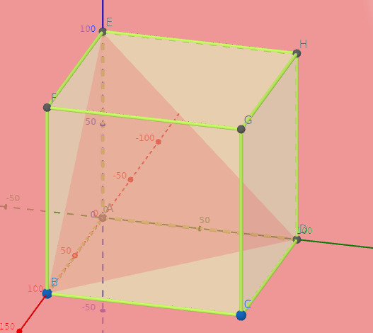
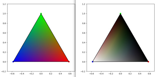
On left, Maxwell triangle for a RGB cube. On right, Maxwell triangle on a HSL cube. Plot code based on this website

So here you have it. The result from these polls will inevitably fall in these. cw spoilers I guess

[govindhtech]

What Is Neural Processing Unit NPU? How Does It Works

What is a Neural Processing Unit?

A Neural Processing Unit NPU mimics how the brain processes information. They excel at deep learning, machine learning, and AI neural networks.

NPUs are designed to speed up AI operations and workloads, such as computing neural network layers made up of scalar, vector, and tensor arithmetic, in contrast to general-purpose central processing units (CPUs) or graphics processing units (GPUs).

Often utilized in heterogeneous computing designs that integrate various processors (such as CPUs and GPUs), NPUs are often referred to as AI chips or AI accelerators. The majority of consumer applications, including laptops, smartphones, and mobile devices, integrate the NPU with other coprocessors on a single semiconductor microchip known as a system-on-chip (SoC). However, large data centers can use standalone NPUs connected straight to a system’s motherboard.

Manufacturers are able to provide on-device generative AI programs that can execute AI workloads, AI applications, and machine learning algorithms in real-time with comparatively low power consumption and high throughput by adding a dedicated NPU.

Key features of NPUs

Deep learning algorithms, speech recognition, natural language processing, photo and video processing, and object detection are just a few of the activities that Neural Processing Unit NPU excel at and that call for low-latency parallel computing.

The following are some of the main characteristics of NPUs:

Parallel processing: To solve problems while multitasking, NPUs can decompose more complex issues into smaller ones. As a result, the processor can execute several neural network operations at once.

Low precision arithmetic: To cut down on computing complexity and boost energy economy, NPUs frequently offer 8-bit (or less) operations.

High-bandwidth memory: To effectively complete AI processing tasks demanding big datasets, several NPUs have high-bandwidth memory on-chip.

Hardware acceleration: Systolic array topologies and enhanced tensor processing are two examples of the hardware acceleration approaches that have been incorporated as a result of advancements in NPU design.

How NPUs work

Neural Processing Unit NPU, which are based on the neural networks of the brain, function by mimicking the actions of human neurons and synapses at the circuit layer. This makes it possible to execute deep learning instruction sets, where a single command finishes processing a group of virtual neurons.

NPUs, in contrast to conventional processors, are not designed for exact calculations. Rather, NPUs are designed to solve problems and can get better over time by learning from various inputs and data kinds. AI systems with NPUs can produce personalized solutions more quickly and with less manual programming by utilizing machine learning.

One notable aspect of Neural Processing Unit NPU is their improved parallel processing capabilities, which allow them to speed up AI processes by relieving high-capacity cores of the burden of handling many jobs. Specific modules for decompression, activation functions, 2D data operations, and multiplication and addition are all included in an NPU. Calculating matrix multiplication and addition, convolution, dot product, and other operations pertinent to the processing of neural network applications are carried out by the dedicated multiplication and addition module.

An Neural Processing Unit NPU may be able to do a comparable function with just one instruction, whereas conventional processors need thousands to accomplish this kind of neuron processing. Synaptic weights, a fluid computational variable assigned to network nodes that signals the probability of a “correct” or “desired” output that can modify or “learn” over time, are another way that an NPU will merge computation and storage for increased operational efficiency.

Testing has revealed that some NPUs can outperform a comparable GPU by more than 100 times while using the same amount of power, even though NPU research is still ongoing.

Key advantages of NPUs

Traditional CPUs and GPUs are not intended to be replaced by Neural Processing Unit NPU. Nonetheless, an NPU’s architecture enhances both CPUs’ designs to offer unparalleled and more effective parallelism and machine learning. When paired with CPUs and GPUs, NPUs provide a number of significant benefits over conventional systems, including the ability to enhance general operations albeit they are most appropriate for specific general activities.

Among the main benefits are the following:

Parallel processing

As previously indicated, Neural Processing Unit NPU are able to decompose more complex issues into smaller ones in order to solve them while multitasking. The secret is that, even while GPUs are also very good at parallel processing, an NPU’s special design can outperform a comparable GPU while using less energy and taking up less space.

Enhanced efficiency

NPUs can carry out comparable parallel processing with significantly higher power efficiency than GPUs, which are frequently utilized for high-performance computing and artificial intelligence activities. NPUs provide a useful way to lower crucial power usage as AI and other high-performance computing grow more prevalent and energy-demanding.

Multimedia data processing in real time

Neural Processing Unit NPU are made to process and react more effectively to a greater variety of data inputs, such as speech, video, and graphics. When response time is crucial, augmented applications such as wearables, robotics, and Internet of Things (IoT) devices with NPUs can offer real-time feedback, lowering operational friction and offering crucial feedback and solutions.

Neural Processing Unit Price

Smartphone NPUs: Usually costing between $800 and $1,200 for high-end variants, these processors are built into smartphones.

Edge AI NPUs: Google Edge TPU and other standalone NPUs cost $50–$500.

Data Center NPUs: The NVIDIA H100 costs $5,000–$30,000.

Read more on Govindhtech.com